
Updated Sep 7, 2026 · Week 1 board.
Three formats, one number
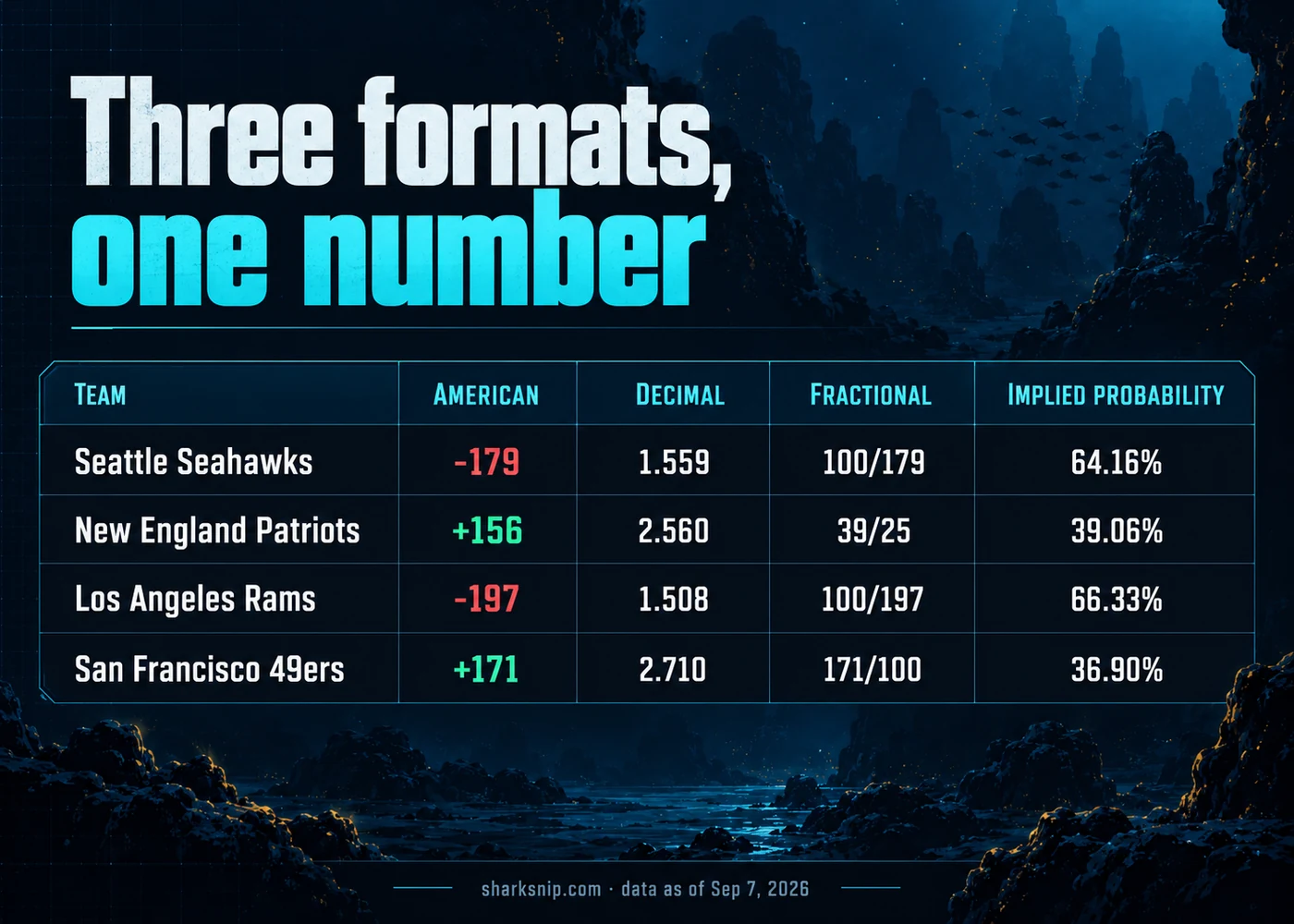
A price is one number wearing whatever clothes the local market puts on it. Pinnacle has the Seahawks at -179 over the Patriots, kickoff Wednesday night, Sep 9. Same book has the Rams at -197 over the 49ers on Thursday night, Sep 10. Both of those are American odds.
Both are Pinnacle's own number. Both convert into the other two formats by arithmetic, never by anybody's opinion. That matters the day a friend texts you a decimal price, or an offshore book quotes you a fraction, and you need to know whether the two of you are looking at the same bet.
Converting a negative price
Negative prices convert off their own size. Drop the minus, then divide the size by itself plus 100. Seattle at -179 gives you 179 / (179 + 100), which is 64.16%. For the decimal, add 1 to 100 divided by that same size: 1 + 100/179 = 1.559.
The fraction is that same 100/179, reduced as far as it will go. 179 shares nothing with 100, so it stays 100/179 against a win.
The Rams' -197 walks the identical three steps, and the table below carries the results: 66.33% implied chance, 1.508 in decimal, 100/197 as a fraction. Put $197 on the Rams at -197 and a winner pays you $100 in profit. Put that same $197 down at decimal odds of 1.508 and you have described the exact same ticket, because $197 times 1.508 is $297.08 coming back to you in total.
Converting a positive price
A positive price flips the arithmetic around. Take 100 and divide it by the price plus 100. New England at +156 gives 100 / (156 + 100), or 39.06%. For the decimal, add 1 to the price over 100: 1 + 156/100 = 2.560.
The fraction is 156/100 reduced, which comes out 39/25.
San Francisco's +171 runs the same way, and the table below has it: 36.90% implied chance, 2.710 decimal, 171/100 fractional, already as low as it reduces because 171 and 100 share nothing but 1. Drop $100 on San Francisco at +171 and a winner returns $271 all in. Which is $100 times 2.710, the same answer arrived at from the other direction.
Which format you're shown mostly tells you where you're standing, not what you're being charged. The three US books on our own screen default to American. Pinnacle. DraftKings.
Bovada. Exchange-style platforms lean decimal instead, and fractional is the older United Kingdom habit. A reader who only ever learned one of the three still owns the same 64.16% on Seattle once the conversion is run. Notation moves around and that 64.16% sits perfectly still.
| Team | American | Decimal | Fractional | Implied probability |
|---|---|---|---|---|
| Seattle Seahawks | -179 | 1.559 | 100/179 | 64.16% |
| New England Patriots | +156 | 2.560 | 39/25 | 39.06% |
| Los Angeles Rams | -197 | 1.508 | 100/197 | 66.33% |
| San Francisco 49ers | +171 | 2.710 | 171/100 | 36.90% |
What the format does and does not change
Writing -179 as 1.559 or as 100/179 does not change the price. It changes which arithmetic is easiest for the job in front of you. Decimal multiplies straight against a stake and hands you the total coming back. Fractional shows the profit ratio against the stake.
American tells you what to risk, or what you'd win, against a flat 100 units. What none of the three does is take the book's cut out of the number. Every chance in that table comes off one side of one book's price. Nobody has looked at the opposite side of that matchup.
So read those four percentages as a book's asking price rather than a fair two-sided number.
The odds converter on the desk will run this three-way swap on any price you type into it. Our Week 1 board carries every price quoted above, at every book on it. And a separate guide on converting free-bet credit handles a related problem that is not this one.
All of this is arithmetic on a pregame price. None of it is a claim about what either of those games does once it kicks off. The broader odds hub has the rest of that same Week 1 board, should you want to try the three-format swap on a price of your own choosing.

The Receipts Drawer
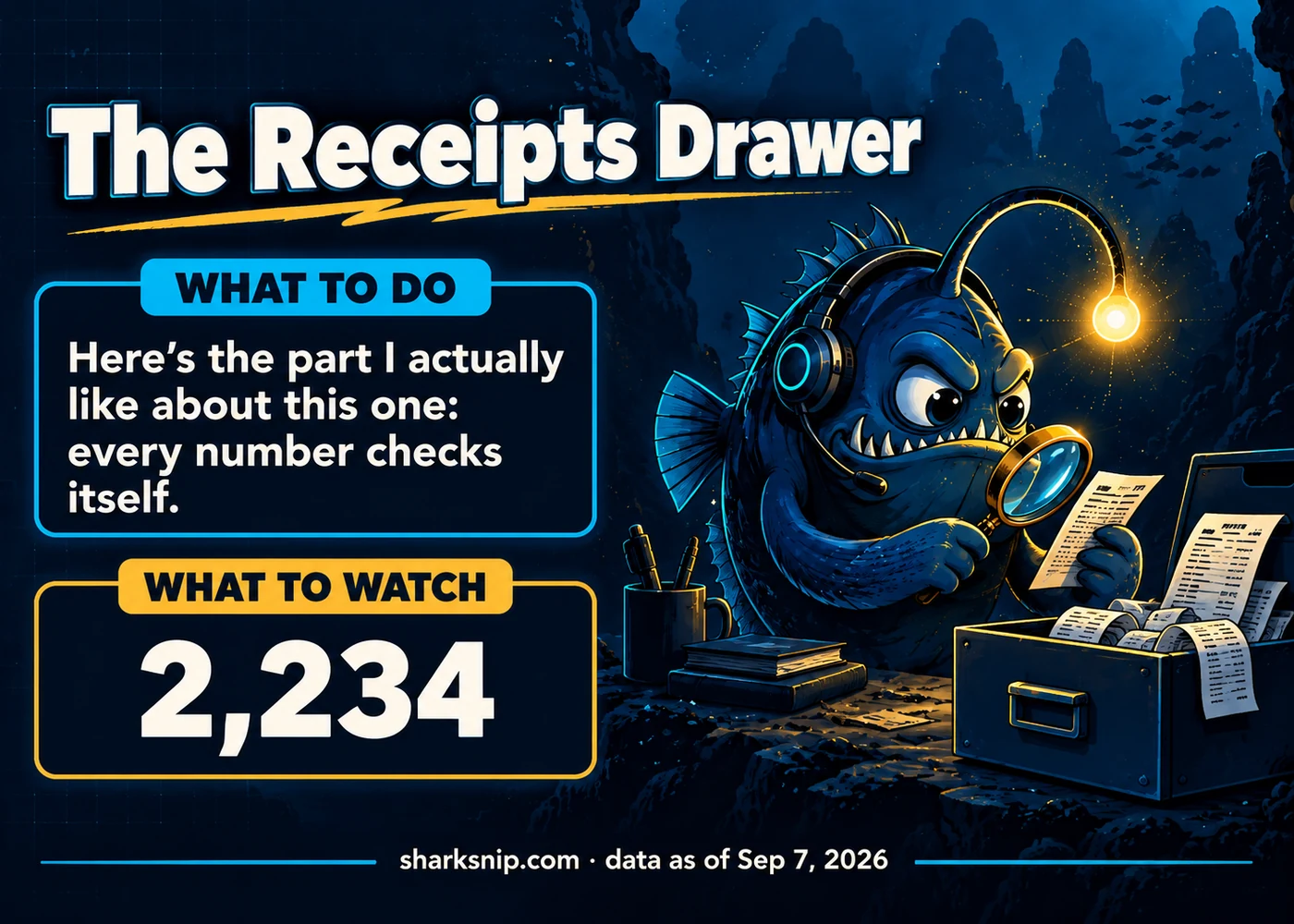
Three costumes, one number: -179, 1.559, 100/179, and 64.16% sitting underneath all three. It comes back identical every time you run it, and I like that about this one. Arithmetic never has a bad week. The honest flag: that 64.16% is Seattle's chance at Pinnacle's asking price alone.
Check it against New England's own price on the same game and the fair number lands lower. So watch the price itself. If Pinnacle comes off -179 before Wednesday night, run the new number back through the same three steps and the percentage moves right along with it.